Each set of states was assigned its own memory, timer and counter address space which allowed for easier monitoring and debugging throughout the program.
Below is a table identifying the way in which resources were allocated:
| Name | Main State | Substates | State Memory | Other Memory | Timers |
| Primary | – | S0-9 | M0.0-3.7 | M4.0-9.7 | T0-9 |
| Powerup | S0 | – | – | – | – |
| Dormant | S1 | S100-199 | M10.0-13.7 | M14.0-19.7 | T10-19 |
| Starting | S2 | S200-299 | M20.0-23.7 | M24.0-29.7 | T20-29 |
| Recover | S3 | S300-349 | M30.0-33.7 | M34.0-34.7 | T30-34 |
| Recover+Run Lights | S3 | S350-399 | M35.0-38.7 | M39.0-39.7 | T35-39 |
| E-Stop | S4 | S400-499 | M40.0-43.7 | M44.0-49.7 | T40-49 |
| Running: Stacking | S5 | S1000-1499 | M100.0-103.7 | M104.0-149.7 | T100-149 |
| Running: Sorting | S5 | S1500-S1999 | M150.0-M153.7 | M140.0-199.7 | T150-199 |
| Recover+Run Lights | S5 | S350-399 | M35.0-38.7 | M39.0-39.7 | T35-39 |
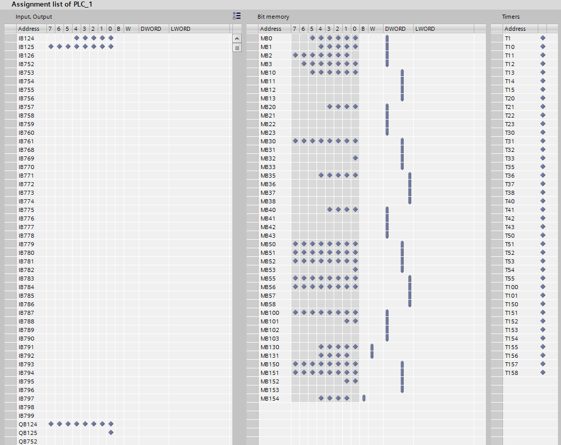
The above table can be seen to align with the below implementation assignment list as extracted from the PLC program.
More information on the utilisation and behaviour of each state/sub-state can be found under Code and Diagrams.